Code
tanks <- function (n_tanks = 47, n_obs = 5, n_reps = 100, fixedest = 50)
{
    temp <- as.matrix(rep(n_tanks, n_reps))
    temp <- apply(temp, 1, sample, size = n_obs)
    temp <- t(apply(temp, 2, tanks.ests, fixedest))
    temp
}The function tanks simulates n_reps battles with n_obs serial numbers recorded for each battle. The argument n_tanks is the number of tanks that the Germans had. The argument fixedest is the expert’s best guess.
tanks <- function (n_tanks = 47, n_obs = 5, n_reps = 100, fixedest = 50)
{
temp <- as.matrix(rep(n_tanks, n_reps))
temp <- apply(temp, 1, sample, size = n_obs)
temp <- t(apply(temp, 2, tanks.ests, fixedest))
temp
}The function tank.ests runs on a sample of observed serial numbers. Each of the vector values is the result of a student supplied estimator. These need to be changed to reflect the class’ ideas.
tanks.ests <- function (x = stop("Argument 'x' is missing"), fixedest = 125)
{
    n <- length(x)
    nodd <- n %% 2 == 1
    ests <- rep(NA, 16)
    xbar <- mean(x)
    xmedian <- median(x)
    xn <- max(x)
    xvar <- var(x)
    xstddev <- sqrt(xvar)
    x1 <- min(x)
    rng <- c(-1,1)%*%range(x)
    xsum <- sum(x)
    xnm1 <- sort(x)[n-1]

    ests[1] <- 2 * xbar
    ests[2] <- 2 * xmedian
    ests[3] <- xn
    ests[4] <- xbar + 2*xstddev
    ests[5] <- xbar + 3*xstddev
    ests[6] <- nodd * (xmedian + x[(n+1)/2 + 1]) + !nodd * (xmedian + x[n/2 + 1])
    ests[7] <- xn + xmedian
    #
      y = sort(x)
      z = c(NA,y[-n])
    ests[8] <- xn + mean(y-z, na.rm = TRUE)
      z = c(0,y[-n])
    ests[9] <- xn + mean(y-z)
      z = c(1,y[-n])
    ests[10] <- xn + mean(y-z)
    ests[11] <- (3*xn - x1)/2
    ests[12] <- (5*xn - xbar)/3
    ests[13] <- 3*xmedian + rng
    ests[14] <- xn
    ests[15] <- xn * ((n+1)/n) - 1
    ests[16] <- fixedest
    names(ests) <- c("2*xbar", "2*m", "x[n]", "xbar+2s", "xbar+3s", "m + next largest",
                     "x[n] + m", "x[n]+mean(x -lag(x))", "x[n]+mean(x -lag(x) w/ 0)",
                     "x[n]+mean(x -lag(x) w/ 1)", "(3x[n]-x[1])/2", "(5*x[n]-xbar)/3",
                     "3m + range(x)", "x[n]", "UMVUE", fixedest)
    ests

    #ests[1] <- xn
    #ests[2] <- 2 * xbar
    #ests[3] <- xn + x1
    #ests[4] <- xn + rng/2
    #ests[5] <- xbar + xstddev
    #ests[6] <- 2 * xmedian
    #ests[7] <- xn + xnm1
    #ests[8] <- 2*xn - x1
    #ests[9] <- xsum
    #ests[10] <- xn * ((n+1)/n) - 1
    #ests[11] <- fixedest
    #names(ests) <- c("x[n]","2*xbar", "x[n]+x[1]", "x[n]+R/2", "xbar+s", "2*m",
    #                 "x[n]+x[n-1]","2x[n]-x[1]","sum(x)", "UMVUE",fixedest)
    #ests
}The function tanks.descriptives computes descriptive statistics for each of the estimators in tanks.ests.
tanks.descriptives <- function (n = 47, obs = 5, reps = 100, fixedest = 50)
{
    temp <- tanks(n, obs, reps, fixedest)
    means <- apply(temp, 2, mean)
    stddevs <- sqrt(apply(temp, 2, var))
    medians <- apply(temp, 2, median)
    bias <- means - n
    mse <- bias^2 + stddevs^2
    t(cbind(means, stddevs, medians, bias, mse))
}The individual estimates computed for the samples from each battle can be plotted. This allows us to compare location and dispersion statistics — center and spread. tanks.plots2 is intended to be an “improved” version of tanks.plots. Both plots use traditional lattice boxplots and there is a ggplot plot as well.
### Load the lattice package
p_load(lattice)

tanks.plots <- function (n = 47, obs = 5, reps = 100, fixedest = 50)
{
    temp <- tanks(n, obs, reps, fixedest)
    tanknames <- attributes(temp)$dimnames[[2]]
    dims <- dim(temp)
    temp <- as.vector(t(temp))
    temp <- cbind(temp, rep(1:dims[2], dims[1]))
    bwplot(factor(temp[, 2], labels = tanknames) ~
        temp[, 1], xlab = "Number of Tanks",
        ylab = "Estimator")
}

tanks.plots2 <- function (n = 47, obs = 5, reps = 100, fixedest = 50)
{
    temp <- tanks(n, obs, reps, fixedest)
    tanknames <- attributes(temp)$dimnames[[2]]
    dims <- dim(temp)
    temp <- as.vector(t(temp))
    temp <- cbind(temp, rep(1:dims[2], dims[1]))
    bwplot(factor(temp[, 2], labels = tanknames) ~
        temp[, 1], xlab = "Number of Tanks",
        ylab = "Estimator", panel = function (x ,
            y , vref = n, ... )
        {
            panel.bwplot(x, y)
            panel.abline(v = vref, lty = 2)
        }, vref = n)
}

p_load(ggplot2)
p_load(tidyverse)
tanks.plots3 <- function (n = 84, obs = 5, reps = 100, fixedest = 87)
{
    temp <- tanks(n, obs, reps, fixedest)
    tanknames <- attributes(temp)$dimnames[[2]]
    dims <- dim(temp)
    temp <- as.vector(t(temp))
    temp <- cbind(temp, rep(1:dims[2], dims[1]))
    temp <- as_tibble(temp)
    names(temp) <- c("Estimate", "Estimator")
    temp$Estimator <- factor(temp$Estimator)
    ggplot(temp, aes(x=Estimator, y=Estimate)) +
      geom_boxplot(alpha=0.7) +
      stat_summary(fun=mean, geom="point", shape=20, size=5, color="red", fill="red") +
      theme(legend.position="none") +
      scale_fill_brewer(palette="Set1") +
      geom_hline(yintercept = n, alpha = 0.5, color = "blue", lty = 1) +
      coord_flip()
}

tanks.plots4 <- function (n = 84, obs = 5, reps = 100, fixedest = 87)
{
    temp <- tanks(n, obs, reps, fixedest)
    temp <- melt(temp)
    names(temp) <- c("RowID","Estimator","Estimate")
    ggplot(temp, aes(x=reorder(Estimator, Estimate, FUN=mean), y=Estimate)) +
      geom_boxplot(alpha=0.7) +
      stat_summary(fun=mean, geom="point", shape=20, size=5, color="red", fill="red") +
      theme(legend.position="none") +
      xlab("Estimator") +
      scale_fill_brewer(palette="Set1") +
      geom_hline(yintercept = n, alpha = 0.5, color = "blue", lty = 1) +
      coord_flip()
}

tanks.plots5 <- function (n = 84, obs = 5, reps = 100, fixedest = 87)
{
    temp <- tanks(n, obs, reps, fixedest)
    temp <- melt(temp)
    names(temp) <- c("RowID","Estimator","Estimate")
    ggplot(temp, aes(x=reorder(Estimator, Estimate, FUN=mean), y=Estimate)) +
      geom_violin(alpha=0.7) +
      stat_summary(fun=mean, geom="point", shape=20, size=5, color="red", fill="red") +
      theme(legend.position="none") +
      xlab("Estimator") +
      scale_fill_brewer(palette="Set1") +
      geom_hline(yintercept = n, alpha = 0.5, color = "blue", lty = 1) +
      coord_flip()
}The class’ estimators can be compared using the functions defined above.
  ### Compute descriptive stats
  t(tanks.descriptives(n = 47, obs = 5, reps = 10000, fixedest = 50))
means stddevs medians bias mse
2*xbar 48.14516 11.571031 48.00000 1.145160 135.20014
2*m 48.10140 17.023910 48.00000 1.101400 291.02658
x[n] 40.09400 6.225531 42.00000 -6.906000 86.45008
xbar+2s 50.67561 8.970541 51.65893 3.675611 93.98072
xbar+3s 63.97713 11.866761 65.09947 16.977127 429.04285
m + next largest 48.15770 18.681251 48.00000 1.157700 350.32940
x[n] + m 64.14470 12.548231 65.00000 17.144700 451.39885
x[n]+mean(x -lag(x)) 48.10440 7.624107 50.00000 1.104400 59.34671
x[n]+mean(x -lag(x) w/ 0) 48.11280 7.470638 50.40000 1.112800 57.04875
x[n]+mean(x -lag(x) w/ 1) 47.91280 7.470638 50.20000 0.912800 56.64363
(3x[n]-x[1])/2 56.11480 9.244018 58.00000 9.114800 168.53145
(5*x[n]-xbar)/3 58.79914 9.245939 61.13333 11.799140 224.70709
3m + range(x) 104.19370 26.563252 105.00000 57.193700 3976.72566
x[n] 40.09400 6.225531 42.00000 -6.906000 86.45008
UMVUE 47.11280 7.470638 49.40000 0.112800 55.82315
50 50.00000 0.000000 50.00000 3.000000 9.00000 ### Plot the estimates from each of the estimators
tanks.plots(n = 47, obs = 5, reps = 10000, fixedest = 50)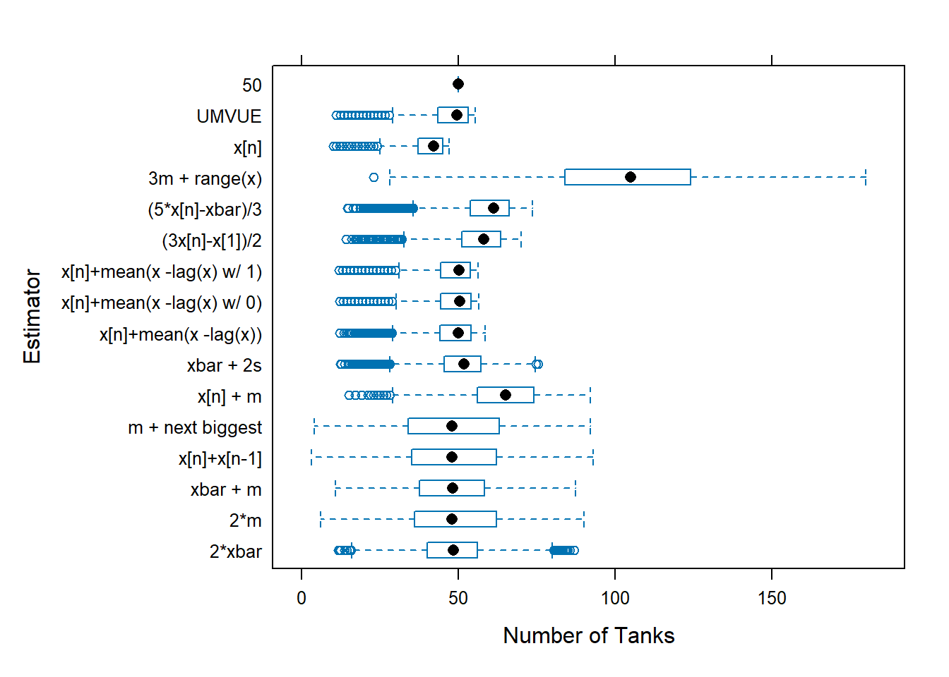
  ### Plot the estimates from each of the estimators
  tanks.plots2(n = 47, obs = 5, reps = 10000, fixedest = 50)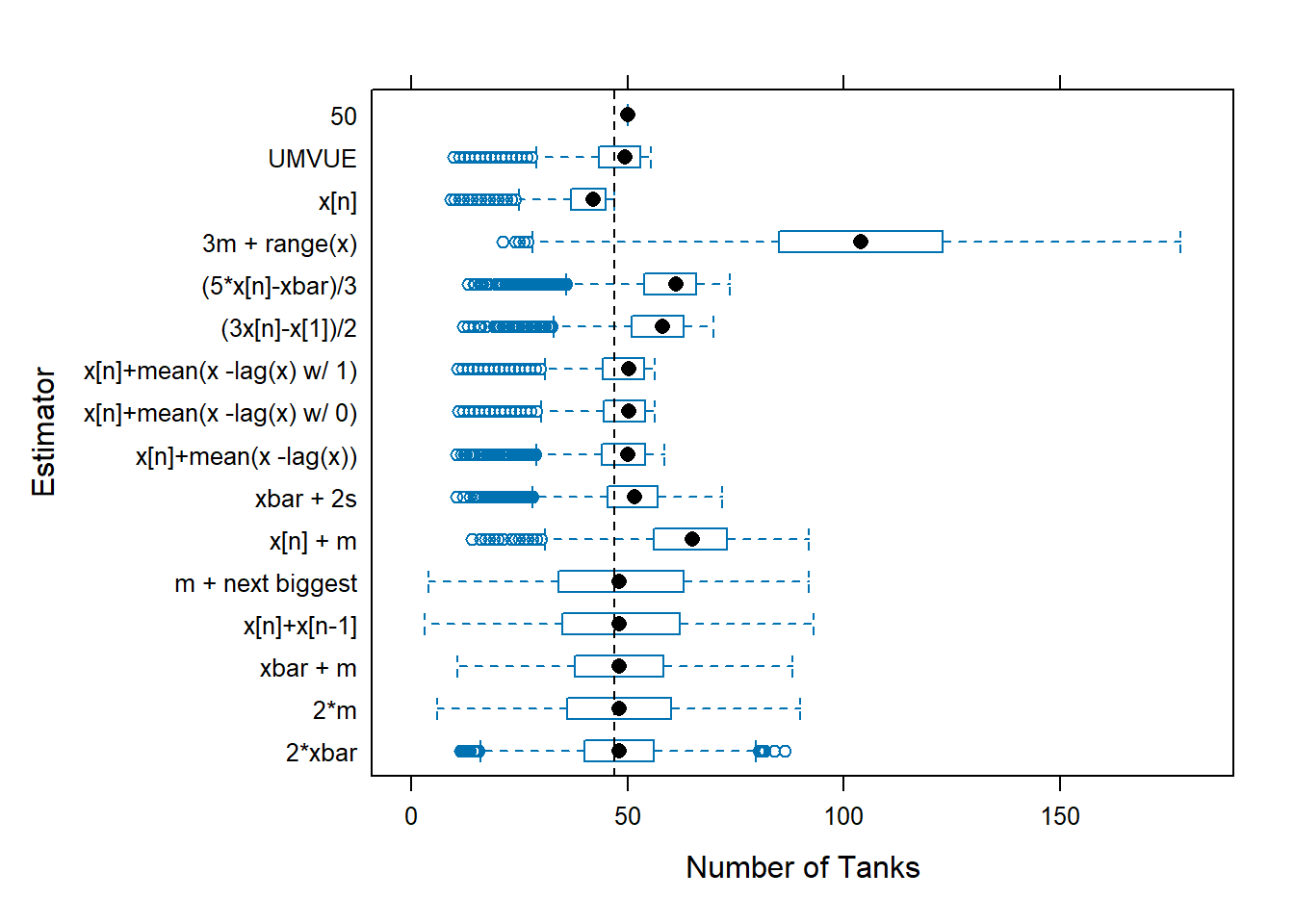
  ### Plot the estimates from each of the estimators
  tanks.plots4(n = 47, obs = 5, reps = 10000, fixedest = 50)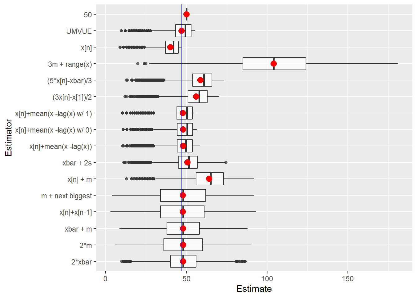
  ### Plot the estimates from each of the estimators
  tanks.plots5(n = 47, obs = 5, reps = 10000, fixedest = 50)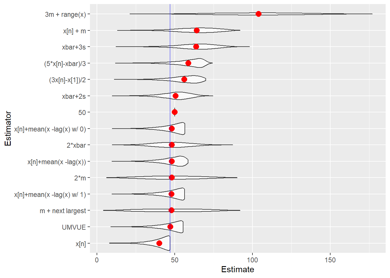
Note that \widehat{N} = X_{(n)} \frac{n+1}{n} - 1 is UMVUE for N when the X_i are i.i.d. DU(1,N).